Same Numbers, Different Stories: Why Data Visualisation Matters
Numbers Don’t Always Tell the Full Story
What if four completely different datasets produced almost exactly the same statistical results?
Imagine receiving four management reports. Each shows the same average, a similar spread of values and almost the same relationship between two measures. It would be tempting to conclude that the underlying situations are much alike.
Organisations make decisions using averages, KPIs, percentages and management reports every day. These numbers are useful: they simplify information and help people track performance. But that simplification can conceal important patterns.
The importance of data visualisation becomes clear when we look beyond the summary. A graph can reveal a curve, an unusual observation or a cluster that a single number cannot describe. The aim is to understand the evidence before deciding what it means.
Four Datasets, Almost Identical Statistics
In 1973, statistician Francis J. Anscombe published Graphs in Statistical Analysis. His recognised demonstration, now called Anscombe’s Quartet, consists of four datasets with 11 observations each.
Each observation contains an X-value and a Y-value. Think of these as two measurements whose relationship we want to explore. For this exercise, they are abstract values rather than sales figures or customer results.
The table below summarises the datasets. Sample standard deviation describes how spread out the observations are. Pearson correlation measures the strength and direction of a linear relationship. The regression equation describes a fitted straight line.
| Statistic | Each dataset |
|---|---|
| Observations | 11 |
| Mean X | 9.00 |
| Mean Y | 7.50 |
| Sample standard deviation X | 3.32 |
| Sample standard deviation Y | 2.03 |
| Pearson correlation | 0.82 |
| Rounded linear regression | Y = 3.00 + 0.500X |
The statistics match at the precision shown, not in every underlying decimal. Correlations are about 0.816: at three decimal places, Datasets I–III round to 0.816 and Dataset IV to 0.817. The orange line used below is the shared rounded equation, rather than four exactly identical fitted lines.
Before looking at the graphs, pause: would you expect these datasets to look similar?
Now Let’s Visualise the Data
These four datasets have almost identical statistics. Do you think their graphs will look the same?
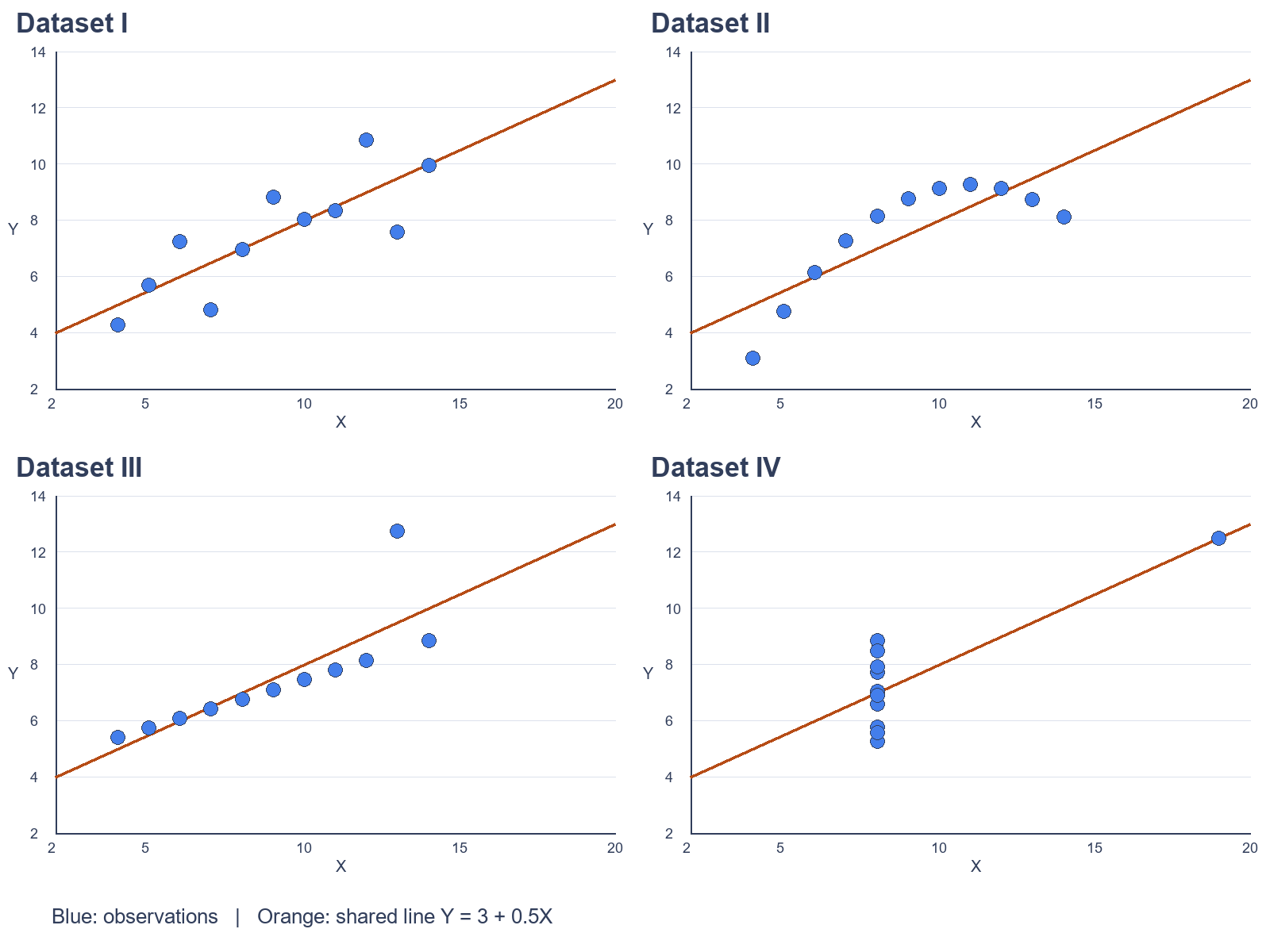
Open the comparison below, then explore each dataset. All charts use the same X-axis range of 2–20 and Y-axis range of 2–14. Blue dots show observations; the orange line shows the shared rounded equation, Y = 3 + 0.5X.
Dataset I — A Relatively Normal Linear Relationship
The points broadly follow a straight line, with some variation around it. Here, a linear regression is a reasonable first description of the relationship.
That does not make the line a perfect prediction or establish cause and effect. It simply means the visual pattern is broadly consistent with the model being used.
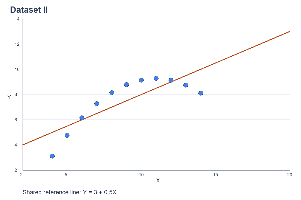
Dataset II — A Curved Relationship
The second dataset follows a clear curve. A straight line misses that shape, even though its summary statistics closely resemble Dataset I.
This matters when interpreting data: a single correlation coefficient cannot tell us whether a relationship bends or changes direction. A different model might be more appropriate after further investigation.
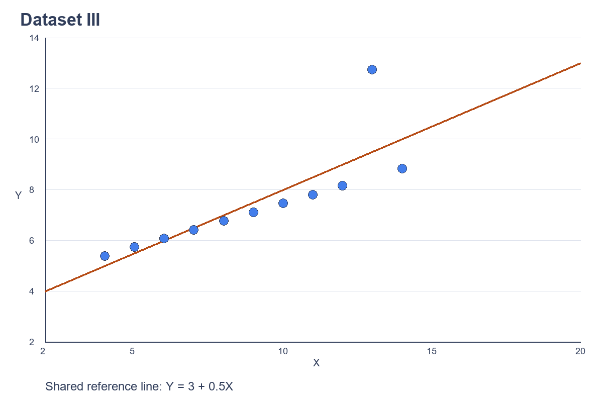
Dataset III — The Impact of an Outlier
Most observations sit very close to a rising straight line. One point, at X = 13 and Y = 12.74, lies well above that pattern and changes the fitted relationship and statistical summary.
The graph gives us a reason to investigate. Is the unusual observation valid, a recording error or evidence of a different situation? Removing it automatically would be as careless as ignoring it.
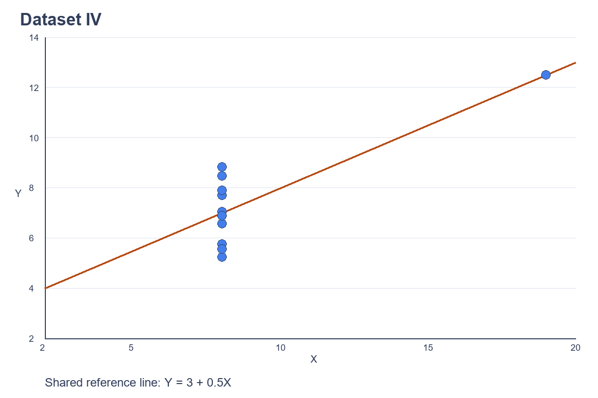
Dataset IV — The Influence of a Single Observation
Ten observations have the same X-value, 8. One observation, at X = 19, supplies almost all the horizontal variation and strongly influences the apparent correlation and regression line.
This is a high-leverage observation: its X-value is far from the others. Without it, the remaining X-values do not vary, so their Pearson correlation is undefined and a meaningful slope cannot be estimated.
Same statistics. Four different stories. More precisely, the summaries are nearly identical; the underlying patterns are profoundly different.
What This Means for Businesses
Anscombe’s Quartet is a statistical demonstration, but its lesson applies to everyday business data. The following examples are illustrative, not reports of Qubytix customer projects.
Sales and revenue. Two businesses might report the same average monthly sales. One could grow steadily while the other experiences pronounced seasonal peaks and quiet periods. A time-series chart helps distinguish these situations before budgeting, staffing or stock decisions are made.
Operational performance. Two systems could have identical average response times. One might respond consistently; the other could suffer occasional severe delays. A distribution chart and response-time percentiles can expose the experience hidden behind the average.
Engineering and sensor data. Similar numerical summaries can conceal different spikes, variations or unexpected responses. Plotting measurements over time, location or operating conditions helps identify where further investigation is needed.
In each case, visualisation suggests patterns and questions. It does not independently prove their causes. Context and additional evidence still matter.
Visualisation Is More Than Making Attractive Charts
Effective data visualisation is not about adding colourful graphs to a presentation. It helps people inspect information and ask better questions before making decisions.
- Identify trends and relationships.
- Detect anomalies and outliers.
- Understand changes over time.
- Compare performance and behaviour.
- Recognise potential data-quality issues.
- Ask better questions before acting.
Data cleaning, sound statistical analysis, subject-matter knowledge and appropriate visualisation work together. A graph cannot rescue unreliable source information, and statistical analysis should not be skipped because a pattern looks convincing.
A misleading chart can be just as problematic as an incomplete summary. Inconsistent axes, unsuitable chart types or selectively chosen periods can distort interpretation. Choose scales deliberately, label measures clearly and show the context readers need.
From Raw Data to Better Decisions
You do not need to start with a large dashboard project. A useful workflow can begin with a specific business question and the information already available:
- Collect and consolidate relevant information from spreadsheets, databases and operational systems.
- Clean and validate records, units, dates and missing values.
- Analyse the statistical characteristics, including averages and variation.
- Visualise patterns, relationships and unusual behaviour.
- Interpret the findings in their business context.
- Use the findings to support informed decisions and identify what to investigate next.
Keep a record of assumptions and data limitations. This makes the reasoning easier to review and the analysis easier to repeat when new information arrives.
How Qubytix Can Help
Qubytix Solutions helps organisations organise, analyse and visualise information through data analytics, business intelligence, reporting dashboards and specialised analytical applications.
The right approach depends on your question and your data. Sometimes a focused analysis is enough. In other cases, repeatable reporting or an ongoing dashboard helps keep useful information visible.
Your business may already have the data it needs. The next step is understanding what that data is telling you.
Explore our Data Analytics & Business Intelligence services or discuss your requirements with our team.
References and Data
Francis J. Anscombe (1973), Graphs in Statistical Analysis, The American Statistician, 27(1), 17–21.
R official documentation: Anscombe’s Quartet. Numerical observations were checked against the Rdatasets CSV copy of R’s anscombe dataset.
All charts were generated specifically for Qubytix from the published datasets. Means, sample standard deviations, correlations and regression coefficients were independently recalculated from the plotted observations.